Introduction to Neural Networks - Linear Classification (Part 2)

Hey there, welcome! This article is the second part of my series on introducing neural networks. The last time we had some fun with simple predictors by teaching them the relationship between miles and kilometers. If you've missed this go ahead and find it here:
 Philipp Zimmermann
Today we will continue our journey with simple linear classifiers. We cover the math behind these algorithms, talk about some training fundamentials and code our own linear classifier using Python.
This series is based on the great book Neuronale Netze selbst programmieren.
Classifiers are similar to predictors
In the first article of this series we learned about predictors. Basically we adjusted one parameter of our neuron based on the error it made during prediction. It's actually very simple to make the jump to linear classifiers. Just think of this one parameter as a linear function.
Last time we predicted a linear relationship between kilometers and miles using our parameter c. Let's visualize it using the following diagram.
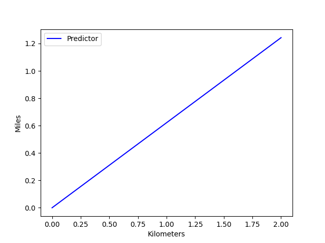
We see that our predictor can be represented as a linear function while y = miles, x = kilometers and m = c.
\( y = x * m \)
\( y = m * x \)
Mathematics of linear classification
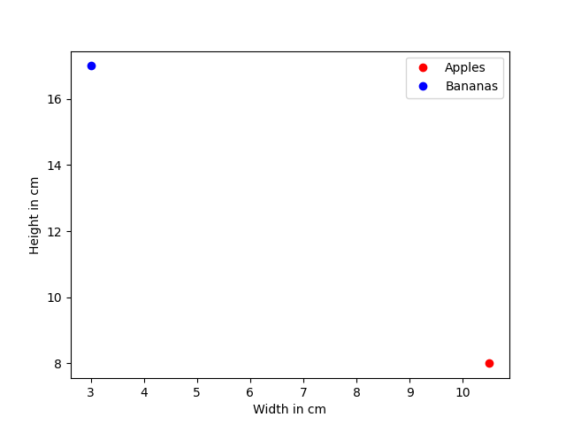
Let's keep this in mind and have a look at another example. This time we have two groups of fruit. First we have bananas which are long and thin and apples which are short and thick. We also have some data collected by measuring an apple and a banana. The data is represented in the table below.
| Fruit | Height (cm) | Width (cm) |
|---|---|---|
| apple | 8.0 | 10.5 |
| banana | 17.0 | 3.0 |
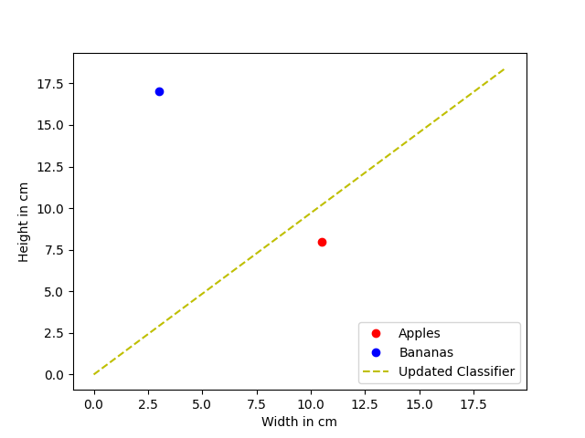
When we visualize our data we get the following diagram with red being apples and blue representing bananas.
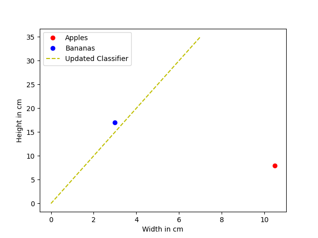
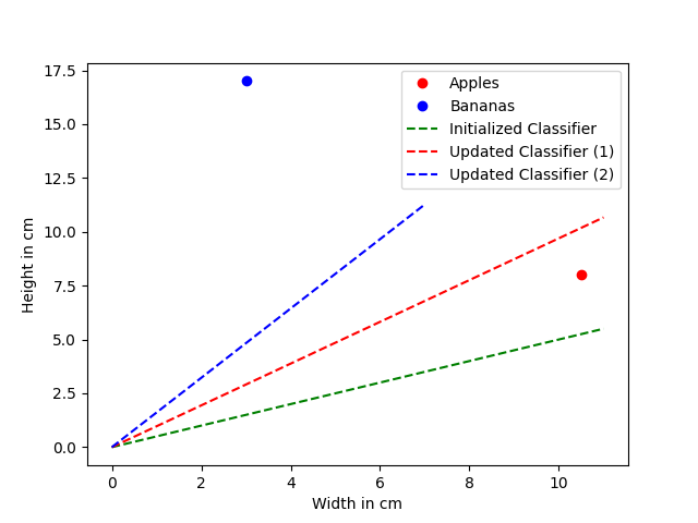
Our goal is to build a classifier who is able to separate the apple from the banana such that if a new datapoint is introduces we can tell which fruit it is. So let us try modelling this in our diagram. Therefore, we initialize a linear classifier with a random value.
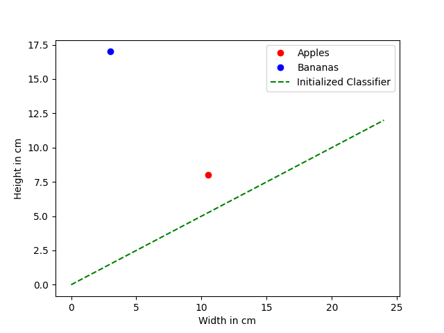
Great. We now have a classifier which devides the diagram in two parts. We initialized it at random (m = 0.5) so we see that it does not work with our provided data yet. At this point our classifier looks like this.
At the end we want a classifier that is able to split the diagram in a way that all apples are on the right side of the line and all bananas are on the left side of the line.
This time we do not use the linear function to predict the relationship between kilometers and miles. Instead we use it to separate our data samples. Again we will adjust the parameter m of the linear function and thus change its slope. There is no further computation needed to see that our randomly initialized function is not a good classifier yet. Let's see how far we're off.
Therefore, we use the apple-datapoint (height = 8.0 and width = 10.5) and put it in our classifier as follows. Remember, height is represented as y and width as x.
\( y = 0.5 * 10.5 \)
\( y = 5.25 \)
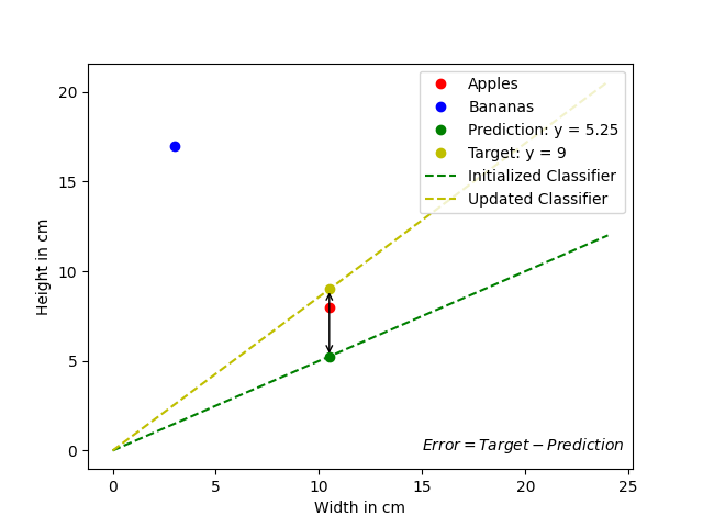
When we apply our classifier to the example above we see that the predicted value y = 5.25 is not accurate. It should have been y = 8.0. So we can calculate the error that has been made. But before we do this, let's think about the value of y for a second. If y = m * 10.5 = 8.0 the linear function would look like this:
However, this is not what we want. We don't want a predictor who takes the width of a fruit as input and predicts the height. We want it to be a classifier separating the two clusters from each other.
That means that our target value is not the height of the apple but a little more. For example we could choose our target value to be y = 9.0.
Now we can calculate the error as follows. In the last part we learned about the error equation:
\( error = 9.0 - 5.25 \)
\( error = 3.75 \)
Let's take a short break and have a look what this means visually.
Now we have the error and we want to use it to adjust m. To do this, we must understand the relationship between these two values.
We know, that our randomly set value for m leads to the wrong value for y. We want m to have the correct value such that y = m * x = target. So we need to adjust m by a certain value. We call this adjustment Δm (delta m). The equation then looks like this:
Remember, that the error is the difference between our target value and our prediction. So let's have a look at the following equations:
\( target = (m + Δm) * x \)
\( prediction = m * x \)
Now we use them to find the relationship between our error and m as follows:
\( error = ((m + Δm) * x) - (m * x) \)
\( error = (m * x) + (Δm * x) - (m * x) \)
\( error = (Δm * x) \)
Great! We found the relationship between them. Let's remember in natural language what we want to achieve.
We want to know how we need to adjust m to be a better classifier. We do this by adding a certain value to m that we call Δm. But we do not know what that value should be. However, we know the error we made by using m. So we want to calculate Δm based on the error. Since we already came up with the upper equation this is very simple now. We only have to rearrange the equation to Δm.
That's it! We found a way to update m based on the prior error we made.
So let's play this through with our prior example of the apple-datapoint (height = 8.0 and width = 10.5). We know the current value for m = 0.5 which produces the result of y = 0.5 * x = 0.5 * 10.5 = 5.25. This leads to an error = target - prediction = 9.0 - 5.55 = 3.75. Now we can calculate Δm.
\( Δm = 0.47 \)
This brings us to our updated classifier:
\( y = (0.5 + 0.47) * x \)
\( y = 0.97 * x \)
Awesome! We just learned from our first training sample and updated the classifier. Now we can continue with our second training sample. Again we will define the new target = 15.
We start by calculating the prediction for the banana-datapoint (height = 17.0 and width = 3.0).
\( prediction = 0.97 * 3 \)
\( prediction = 2.91 \)
Based on the prediction we continue calculating the error.
\( error = 15 - 2.91 \)
\( error = 12.09 \)
We use this error to calculate our adjustment Δm.
\( Δm = 12.09 / 3 \)
\( Δm = 4.03 \)
And finally we can update our classifier and visualize it.
\( y = (0.97 + 4.03) * x \)
\( y = 5 * x \)
Wait a minute! What has just happened? The training process didn't go as we had hoped. The classifier did not separate the space between these two datapoints correctly. Let's investigate our training process.
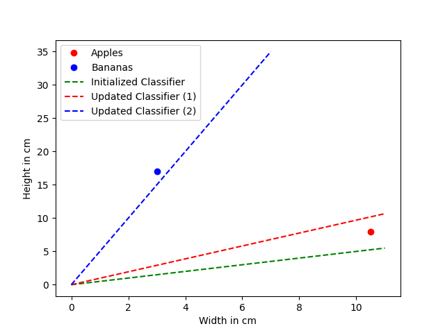
Well, actually we got what we asked for. The classifier is updated by every target value. However, we implemented this in a way, that it always "forgets" about the prior training samples it has already been trained on.
To fix this problem we will introduce a new parameter called learning rate or short lr. This parameter is a hyper parameter since we define it at the beginning and it influences how well the classifier will perform. It takes care of our classifier being able to "remember" prior datapoints it has been trained on. The learning rate is a value between 0 and 1 and is used during the calculation of Δm. Currently we were training using a learning rate of 1, since we only focused on our last datapoint.
Let us begin setting lr = 0.5. And we start over training the classifier by calculating the prediction for the apple-datapoint using our initialized classifier.
\( y = 0.5 * 10.5 \)
\( y = 5.25 \)
We calculate the error based on this prediction. But instead of setting our target value to 9.0 we use the actual value for the apples height which is 8.0.
\( error = 8.0 - 5.25 \)
\( error = 2.75 \)
Now we compute the adjustment Δm by using our new learning rate of lr = 0.5.
\( Δm = 0.5 * (2.75 / 8) \)
\( Δm = 0.5 * 0.34 \)
\( Δm = 0.17 \)
We update our classifier.
\( y = (0.5 + 0.17) * x \)
\( y = 0.67 * x \)
And we continue with training on the second example. Let's calculate the prediction.
\( prediction = 0.67 * 17.0 \)
\( prediction = 11.39 \)
Now we compute the error we made using the prediction.
\( error = 17.0 - 11.39 \)
\( error = 5.61 \)
And we calculate the adjustment Δm again with our new learning rate of lr = 0.5.
\( Δm = 0.5 * (5.61 / 3) \)
\( Δm = 0.5 * 1.87 \)
\( Δm = 0.94 \)
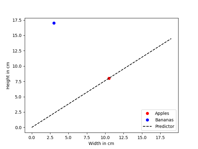
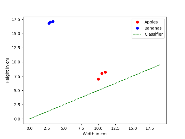
And finally we update our classifier one more time and visualize it.
\( y = (0.67 + 0.94) * x \)
\( y = 1.61 * x \)
That is looking good!
Even with those basic training samples and an easy update function we were able to find a good linear function that can separate them. Of course the classifier will get better with increasing amount of data points and thats why we will use some more in the following implementation phase.
Implementing a linear classifier
This code block implements the procedure from above.
#!/usr/bin/python3
import matplotlib.pyplot as plt
from random import shuffle
class LinearClassifier:
def __init__(self):
"""
Initialize LinearClassifier.
"""
self.lr = 0.05
self.m = 0.5
self.epochs = 5
# Training data (height, width)
self.training_data = {
"apple": [(8.0, 10.5), (7.0, 10.0), (8.2, 11)],
"banana": [(17.0, 3.0), (16.8, 2.8), (17.1, 3.4)]
}
# Testing data (height, width)
self.testing_data = {
"apple": [(6.0, 8.5), (7.8, 9.3), (9.0, 9.0)],
"banana": [(14.0, 2.0), (15.9, 3.8), (19.0, 3.6)]
}
def train(self):
"""
This function trains the classifier.
"""
# Sample training set
train = self.training_data["apple"] + self.training_data["banana"]
shuffle(train)
# Train on training data for iteration times
for epoch in range(self.epochs):
for (height, width) in train:
# Classifier prediction
prediction = self.m * width
# Error
error = height - prediction
# Update parameter
delta_m = error / width
self.m += self.lr * delta_m
# Print training step
print(f"[ Epoch {epoch+1:2.0f}/{self.epochs} ] m: {self.m}")
def classify(self, height, width):
"""
This function classifies the given sample.
"""
prediction = self.m * width
return "apple" if height <= prediction else "banana"
def test(self):
"""
This function is testing the classifier.
"""
for label, datapoints in self.testing_data.items():
correct = 0
for (height, width) in datapoints:
predicted_label = self.classify(height=height, width=width)
if predicted_label == label:
correct += 1
print(f" > {label.capitalize()}:\t{correct:2.0f}/{len(datapoints)} classified correctly")
def visualize(self, visual_name, apples, bananas, graph_len=20):
"""
This function visualizes the given data.
"""
plt.clf()
apple_height = [height for (height, _) in apples]
apple_width = [width for (_, width) in apples]
banana_height = [height for (height, _) in bananas]
banana_width = [width for (_, width) in bananas]
plt.plot(apple_width, apple_height, "ro", label="Apples")
plt.plot(banana_width, banana_height, "bo", label="Bananas")
x = [i for i in range(graph_len)]
y = [i * self.m for i in x]
plt.plot(x, y, "g--", label="Classifier")
plt.ylabel('Height in cm')
plt.xlabel('Width in cm')
plt.legend()
plt.savefig(visual_name)
if __name__ == "__main__":
# Create the classifier
classifier = LinearClassifier()
# Visualization of initialized classifier
classifier.visualize(
visual_name="initialized_classifier",
apples=classifier.training_data["apple"],
bananas=classifier.training_data["banana"],
graph_len=20
)
# Training the classifier
print("--- Training ---\n")
classifier.train()
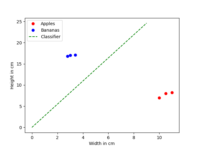
# Testing and visualization of trained classifier
print("\n\n--- Classifiers' prediction after the training ---\n")
classifier.test()
classifier.visualize(
visual_name="trained_classifier",
apples=classifier.training_data["apple"],
bananas=classifier.training_data["banana"],
graph_len=10
)linear_classifier.py
To run the code copy the content and save it to a file called linear_classifier.py. Then you can run the code with the following command.
python3 linear_classifier.pyYou should see the following output in your terminal as well as two created files named initialized_classifier.png and trained_classifier.png.
--- Training ---

[ Epoch  1/5 ] m: 1.2536066102045933
[ Epoch  2/5 ] m: 1.8075767180873854
[ Epoch  3/5 ] m: 2.214795652040682
[ Epoch  4/5 ] m: 2.5141389880987077
[ Epoch  5/5 ] m: 2.7341838469475963


--- Classifiers' prediction after the training  ---

  > Apple:       3/3 classified correctly
  > Banana:      3/3 classified correctly
Conclusion
I hope you had fun today. Again we learned a lot! We saw that even simple datasets and a simple update function are sufficient to train a linear classifier such that it is able to perfectly separate them. We also learned to implement this procedure using Python and to visualize our data.
In the next article we dive deep into the world of neural networks the first time. We start investigating neurons in detail and how we can implement them in Python. Stay tuned and have a great day.
Philipp Zimmermann
Citation
If you found this article helpful and would like to cite it, you can use the following BibTeX entry.
@misc{
	hacking_and_security,
	title={Introduction to Neural Networks - Linear Classification (Part 2)},
	url={https://hacking-and-security.cc/introduction-to-neural-networks-part-2},
	author={Zimmermann, Philipp},
	year={2024},
	month={Jan}
}