By Philipp Zimmermann in Introduction to Neural Networks — Jan 13, 2024

Introduction to Neural Networks - The Neural Network (Part 3)

AI generated image by DALL·E

Welcome! This is the third part of my series on introducing neural networks. In the last post we learned about linear classification by separating apples from bananas. If you have missed it, feel free to check it out.

However, today we will take a look at simple neural networks. We want to understand how predictions are made and how we can influence the decisions of a neural network.

This series is based on the great book Neuronale Netze selbst programmieren.

The biological neuron

For centuries, scientists tried to immitate the biological brain because of its problem solving capabilities. We already know that a brain consits of a huge amount of neurons (100 billion - source) that are connected with each other.

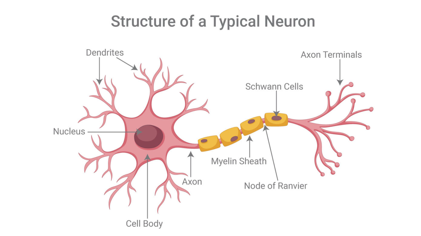
**Figure 1:** Source (last checked on 13 Jan. 2024)

Although there exist some different forms of neurons all take electrical signals as input (dendrites), process them and forward them to the connected neurons (axon terminals). Observations suggest that neurons do not forward the signal right away. Instead it only fires if a specific threshold is reached. You can think of this process like having a cup which gets filled with water (the input signals of the neuron). At a certain point, there is so much water in the cup that the next drop of water causes it to overflow (the neuron fires). Let's see a diagram visualizing this behavior.

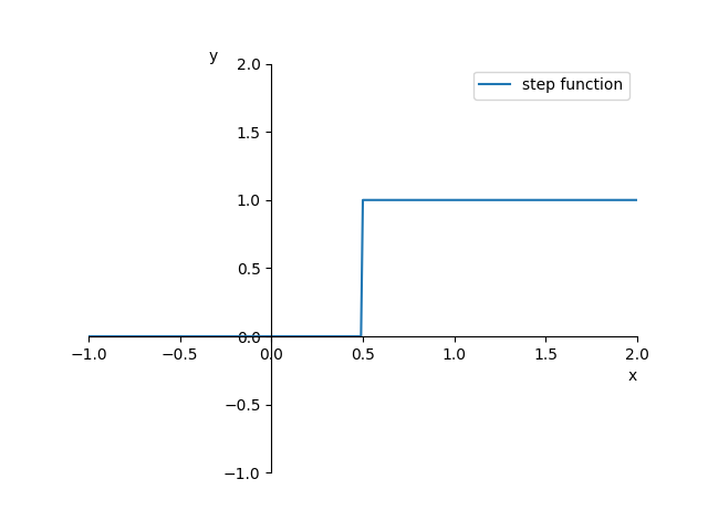
**Figure 2:** Visualization of the step function

What we can see here is the so called step function. Until a specific threshold is reached - 0.5 in our case - it produces zero as output. However, after that the output is one all the time.

So basically this process can be modeled as mathematical function that only produces output when a specific threshold of their inputs is reached. We call this type of function activation function and its job is to "decide" whether the neuron fires or not. If you are interested which activation functions are commonly used you can have a look at this article below.

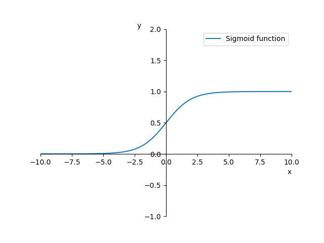
Unfortunately the real world is not as easy as our step function suggests. There is no hard limit that must be reached for the neuron to fire. Instead, this is a smooth process. There are many ways of modelling this behavior by using different activation functions. In this series we will use the Sigmoid activation function, which is popular in the world of classification tasks.

\( y = Sigmoid(x) = \frac{1}{1 + e^{-x}} \)

In this equation e is the Euler's number which is e = 2.71828.... Note that if x = 0 the equation turnes out to be y = 0.5 since every number raised to the power of zero equals one. Thus making y = 1 / (1 + 1) = 0.5. Therefore, the Sigmoid function intersects the y-axis at 0.5. Let's visualize it.

**Figure 3:** Visualization of the Sigmoid function

Great! Now we need to note, that biological neurons not only have one single input. Instead they have multiple ones. So let's see what we can do with this information.

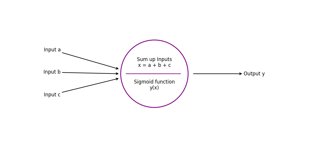
**Figure 4:** Visualisation of an artificial neuron

Here we have an artificial neuron that takes 3 values as input (a, b and c). It calculates the sum and computes the output by using the Sigmoid function. As said before, our brains consist of many neurons. This means that our artificial neural network must also contain multiple neurons. So let's build our first artifial neural network.

**Figure 5:** Artificial neural network with 3 layers

Here we have our first artificial neural network. It consists of 3 layers with 3 neurons each. We call this one a Multi-Layer-Perceptron or a Fully-Connected Neural Network. This is why every neuron of the prior layer is connected to every neuron of the next layer. Note that the neurons in the first layer each have one input and 3 outputs. The third layer on the other hand is a little different. Here each neuron has three input signals and only produces one single output value.

When we now think about what this neural network will do in the future we know that we will provide some input to it. In our case this would be 3 values - one for each input neuron.

Each neuron in the first layer will just forwards the value to the next layer.
Each neuron in the second layer will now sum up all inputs - which are 3 in our case since the prior layer had 3 neurons. After that the result is computed using the Sigmoid function and is sent to each neuron of the next layer.
Each neuron in the last layer will again sum up all 3 inputs. It then computes the result using the Sigmoid function and provides the output.

This means that our input could for example be inputs = [3, 5, 2] and the output could then look like this output = [0.54, 0.23, 0.6].

Alright this looks pretty cool but what exactly is happening here? How does this thing learn? Is there some parameter that can be trained to make better predictions? Yes there is and it's kind of intuitive. We will use the connections of the network.

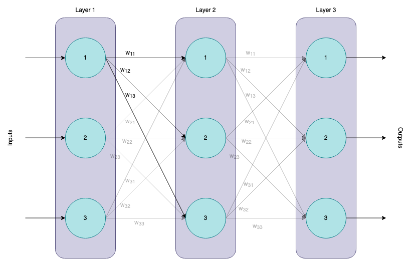
**Figure 6:** Weights in a neural network

Above I highlighted the weights for the first neuron in the first layer. We call them w_11, w12 and w13 based on their source and destination in the specific layers.

Let us now follow the signals through the neural network once more but this time having the weights in place.

Again we will start by providing 3 input values which will be forwarded by each neuron to the next layer. However, this time the input values will be multiplied by the corresponding weights.
Each neuron in the second layer will now sum up all inputs and compute the result using the Sigmoid function afterwards. Again the results are multiplied with the correct weights before sending it to the next layer.
The neurons in the last layer will sum up everything and compute the result using the Sigmoid function. However, this time there are no weights so the output is not changed anymore.

Alright. So we just saw how we can influence the behavior of the neural network with our weights. This gives us the chance to train our model by adjusting the weights of a neural network just like we did in the previous parts with only one paramter.

For better understaning this process we will now create a smaller network which only consists of 4 neurons in two layers and we calculate each operation step by step.

Figure 7: Multi-Layer-Perceptron with 2 layers

Let our input values be inputs = [0.1, 0.5] and let our weights be set as w_11 = 0.3, w_12 = 0.2, w_21 = 0.4 and w_22 = 0.1.

We will start with the equation for the output of the first neuron in the output layer.

\( out_1 = Sigmoid((input_1 * w_{11}) + (input_2 * w_{21})) \)
\( out_1 = Sigmoid((0.1 * 0.3) + (0.5 * 0.4)) \)
\( out_1 = Sigmoid(0.03 + 0.2) \)
\( out_1 = Sigmoid(0.23) \)
\( out_1 = \frac{1}{1 + e^{-0.23}} \)
\( out_1 = 0.56 \)

Let's break this down. We know that the inputs for our first neuron in the output layer is calculated by the input values multiplied by the corresponding weights. This means we need input_1 * w_11 and input_2 * w21. We then sum up the results and apply the Sigmoid function on it. The result is the first output out_1.

We then follow the same steps to compute the output of the second neuron:

\( out_2 = Sigmoid((input_1 * w_{12}) + (input_2 * w_{22})) \)
\( out_2 = Sigmoid((0.1 * 0.2) + (0.5 * 0.1)) \)
\( out_2 = Sigmoid(0.02 + 0.05) \)
\( out_2 = Sigmoid(0.08) \)
\( out_2 = \frac{1}{1 + e^{-0.08}} \)
\( out_2 = 0.52 \)

Let's break it down one more time. We know that the inputs for our second neuron in the output layer is calculated by the input values multiplied by the corresponding weights. This means we need input_1 * w_12 and input_2 * w22. We then sum up the results and apply the Sigmoid function on it such that the result is the second output out_2.

Well done! We just calculated the signal processing of an artificial neural network.

When I was at this point the very first time, I was wondering what this actually meant. I did not get how this will classify something at the end. Since I struggled with that I thought I lose some words on that before we continue with todays implementation.

Interpreting the results of neural networks

What we saw above was the raw output of a neural network. We provided some input and got some output.

Machines are great at calculating stuff and this is what we are using them for. That is why we need to preprocess our data when we want to apply machine learning to a problem. In the last part we used fruits as an example. Each fruit was described by two values the height and the width. This information is representing the fruit in our model. That means, the input to our neural network would be inputs = [height, width].

I think to this point everything should be clear. But what about the output? How should we interprete it. Actually, this is very simple as well. We define how we want to interprete the output.

In our example we could do this: Because we have two output neurons each can represent one fruit. Let's say the first one stands for apples and the second one for bananas. Now we need to match the output values to our labels. This can be done in multiple ways.

For example we could use the Softmax activation function. Then the neurons would tell us the probability that the provided input corresponds to the specific fruit. So if we get outputs = [0.3, 0.7] this would mean, that the neural network is 30% sure that the input was an apple and that it is 70% sure that the input was a banana.

However, we use the Sigmoid activation function. This means, that we can just say, that the neuron with the highest output represents the networks decision. So if we get outputs = [0.777, 0.145] this would mean, that the neural network classified the input as apple. Again if you want to learn more about specific activation functions you can just continue reading here.

Implementing a neural network

This code block implements the procedure from above.

#!/usr/bin/python3

import numpy as np

class NeuralNetwork:

    def __init__(self):
        """
        Initialize NeuralNetwork.
        """
        # Weights
        self.w_11 = 0.3
        self.w_12 = 0.2
        self.w_21 = 0.4
        self.w_22 = 0.1

        # Inputs
        self.inputs = [0.1, 0.5]
    
    def sigmoid(self, x):
        """
        This function implements the Sigmoid activation function.
        """
        return 1 / (1 + np.exp(-x))

    
    def forward(self):
        """
        This function performs the forward step of the neural network.
        """
        outputs = [
            self.sigmoid((self.inputs[0] * self.w_11) + (self.inputs[1] * self.w_21)),
            self.sigmoid((self.inputs[0] * self.w_12) + (self.inputs[1] * self.w_22))
        ]
        return outputs

if __name__ == "__main__":

    nn = NeuralNetwork()
    print(nn.forward())

To run the code copy the content and save it to a file called neural_network.py. Then you can run the code with the following command.

python3 neural_network.py

You should see the following output in your terminal.

--- Neural Network Outputs ---

  > out_1 = 0.56
  > out_2 = 0.52

Conclusion

Today was huge! We built our first neural networks and calculated the signal processing through them. We learned about activation functions and how we need to interpret the results of artificial neural networks.

Next time we will dive deep into matrix multiplication and how this mathematical operation can help us on our journey.

Citation

If you found this article helpful and would like to cite it, you can use the following BibTeX entry.

@misc{
	hacking_and_security, 
	title={Introduction to Neural Networks - The Neural Network (Part 3)}, 
	url={https://hacking-and-security.cc/introduction-to-neural-networks-part-3}, 
	author={Zimmermann, Philipp},
	year={2024}, 
	month={Jan}
}